Table of Contents
- Frequently Asked Questions
- Supported Images
- Image & Mask Loading
- Image Visualization
- Tab Docking
- Coordinate definition (Seed-point initialization)
- Label Annotation/Drawing Panel
- Keyboard Shortcuts
- Utilities (Command-line only)
- Pre-processing
- Segmentation
- Feature Extraction
- Specialized Applications
- Command Line Usage
For Download/Installation Instructions, please see the following:
For Frequently Asked Questions, please see the dedicated FAQ section.
CaPTk has been designed as a modular platform, currently incorporating components for:
- User interaction (e.g., coordinate definition, region annotation, and spherical approximation of abnormalities)
- Pre-processing (e.g., smoothing, bias correction, co-registration, normalization)
- Segmentation
- Feature Extraction
- Specialized Applications
The components of interaction and pre-processing are available for all integrated applications giving a researcher (whether clinical or computational) a single point of entry and exit for all their tasks.
Several CaPTk algorithms and tools can be used from the web on the CBICA Image Processing Portal.
The following sections give a high-level overview of CaPTk, with the intention of familiarizing a new user with the platform functionalities and interface.
Frequently Asked Questions
Please see the dedicated FAQ section.
Supported Images
Currently, CaPTk supports visualization of MR, CT, PET, X-Ray and Full-field Digital Mammography (FFDM) images in NIfTI (i.e., .nii, .nii.gz) format. DICOM (i.e., .dcm) support is limited to a few protocols for MR, CT and MG modalities. In NIfTI format, for MRI, the following modalities are currently supported (the image modality box equivalent is shown in parenthesis):
| Acronym | Image Type |
|---|---|
| T1 | Native T1-weighted MR Image |
| T1Gd | Post-contrast T1-weighted MR Image (also known as T1c, T1-CE) |
| T2 | Native T2-weighted MR Image |
| FLAIR | T2-weighted Fluid Attenuated Inversion Recovery MR Image |
| DSC-ap-rCBV | automatically-extracted proxy to relative Cerebral Blood Volume |
| PERFUSION | Dynamic Susceptibility Contrast-enhanced MR Image (also known as DSC) |
| DTI | Diffusion Tensor Image |
| DWI | Diffusion Weighted Image |
| REC | Recurrence Maps |
* These modalities are currently visualized only within the "Confetti" application.
In addition, CaPTk offers the ability to extract and visualize commonly used measurements from DTI [1] and DSC-MRI, while accounting for leakage correction [2]. The exact measurements supported are:
| Acronym | Image Type |
|---|---|
| DTI-FA | Fractional Anisotropy |
| DTI-AX | Axial Diffusivity |
| DTI-RAD | Radial Diffusivity |
| DTI-TR | Trace |
| DSC-ap-rCBV | automatically-extracted proxy to relative Cerebral Blood Volume |
| DSC-PH | Peak Height |
| DSC-PSR | Percentage Signal Recovery |
References:
- J.M.Soares, P.Marques, V.Alves, N.Sousa. "A hitchhiker's guide to diffusion tensor imaging", Front Neurosci. 7:31, 2013, DOI: 10.33 fnins.2013.00031
- E.S.Paulson, K.M.Schmainda, "Comparison of dynamic susceptibility-weighted contrast-enhanced MR methods: recommendations for measuring relative cerebral blood volume in brain tumors", Radiology. 249(2):601-613, 2008, DOI: 10.1148/radiol.2492071659
Image & Mask Loading
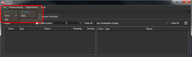
The File -> Load -> Images menu is used to load all image types. Images can also be loaded by dragging and dropping onto the application. In case of DICOM images, loading/dragging a single image loads the entire dicom series.
Mask must be loaded via File -> Load -> ROI menu and also by dragging and dropping onto the application.
For every loaded NIfTI image, the modality is automatically assigned using information from the filename. To assign modalities for DICOM images, or in case of a discrepancy in the modality of a NIfTI image, the user can use the drop-down modality switcher (see below) to revise the modality accordingly. This is typically needed in the Specialized Applications.
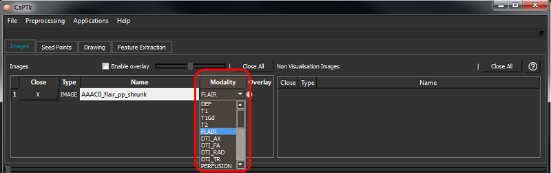
Image Visualization
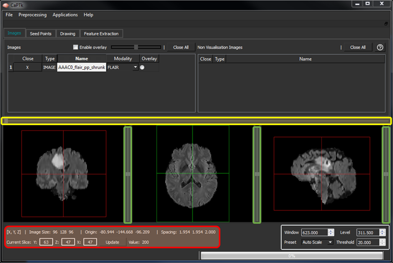
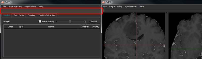
Sliders on each visualization panel (highlighted in green in the figure below) control the movement across respective axes. Note that in DSC-MRI, the single horizontal slider (highlighted in yellow) moves across the time of the acquired dynamic scan.
Various adjustments are available to the user, including:
- Window/Level: right mouse button press + horizontal/vertical mouse move on any visualization panel, respectively.
- Manual Window/Level and setting of different visualization presets: bottom-right panel.
- Image zoom: Ctrl + mouse wheel.
- Image pan: Ctrl + left mouse button press + mouse move.
The bottom-left panel of CaPTk (highlighted in red) shows basic information about the image and the position of the cross-hair. In the visualization panes, the "Z" axis is the center; and "Y" and "X" are to its left and right, respectively. "Z" represents the Axial view for RAI-to-LPS images.
The "Overlay" functionality enables the visualization between two loaded images:
- Double-click one of the two images you want to visualize and then click on its corresponding "overlay" radio button, on its right-most column.
- Click on the "overlay" radio button of the second image that you want to visualize.
- Both "Overlay" and "Underlay" images are now visualized with 50% opacity.
- Check the tick box "Change Opacity".
- Moving the slider changes the opacity between the "Overlay" and the "Underlay" images.
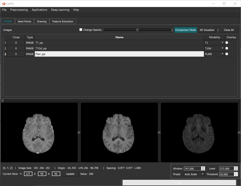
The "Comparison Mode" puts the loaded images (3 maximum) side-by-side for easy visualization along the same axis.
Tab Docking
Double clicking on the tab bar will dock/undock the entire section, resulting in larger visualization panels in your monitor. This behavior is replicated by single click of the dock/undock button at the end of the section as well.
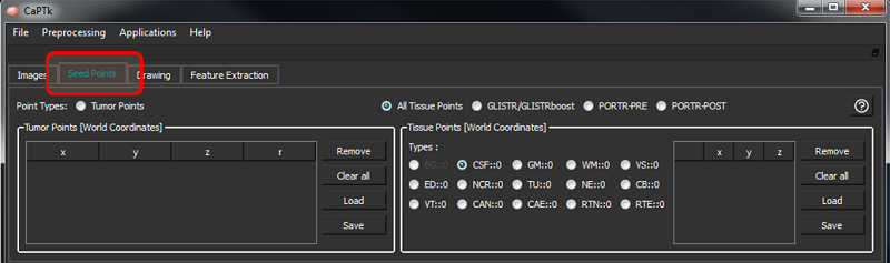
Coordinate definition (Seed-point initialization)
The Seed Points tab includes two general types of initialization (i.e., tumor and tissue points), controlled by the respective radio buttons.
Loading and saving is done via text files in a format consistent with respective applications. Seedpoint files are needed for the following applications (and all derivatives): GLISTR (https://www.cbica.upenn.edu/sbia/software/glistr/) [1-3], GLISTRboost (BraTS 2015 top-ranked algorithm - https://www.med.upenn.edu/sbia/glistrboost.html) [4-6], and PORTR (https://www.cbica.upenn.edu/sbia/software/portr/) [7].
The controls to add/remove points are the shown below.
Tumor Points
These are seed-points used to approximate a tumor by a parametric spherical model, using a seed-point for its center and another for defining its radius. These are helpful for applications like tumor growth model estimation as currently incorporated in GLISTR and GLISTRboost. The controls are as follows:
| Key Stroke | Function/Action |
|---|---|
| Shift + Space | [SEED POINT] Set initial tumor center |
| Control + Space | [SEED POINT] Update tumor radius; on macOS, this is "Fn + Command + Space" |
| Space | [SEED POINT] Update tumor center |
Tissue Points
These are seed-points with coordinate information. They can be used for a multitude of applications where manual initialization(s) are required for a semi-automated algorithm, e.g, segmentation. At the moment these points are being assigned various brain tissue labels, as follows:
| Tissue Acronym | Full Form |
|---|---|
| CSF | Cerebrospinal Fluid |
| VT | Ventricular Cerebrospinal Fluid |
| GM | Gray Matter |
| WM | White Matter |
| VS | Vessels |
| ED | Edema |
| NCR | Necrosis |
| ET | Enhancing Tumor |
| NE | Non-Enhancing Tumor |
| CB | Cerebellum |
| CAE | Enhancing Cavity |
| CAN | Non-Enhancing Cavity |
| RTN | Tumor Recurrence |
| RTE | Enhanced Tumor Recurrence |
Application-specific tissue types are automatically enabled when the corresponding application is selected. For example, when trying to initialize tissue points for GLISTR/GLISTRboost, only CSF, GM, WM, VS, ED, NCR, TU, NE and CB buttons will be enabled and the rest will be disabled. If there are some required tissue types missing for an application, CaPTk will display a warning and not let the user save an incomplete set of tissue points.
References:
- A.Gooya, K.M.Pohl, M.Billelo, G.Biros, C. Davatzikos, "Joint segmentation and deformable registration of brain scans guided by a tumog rowth model", Med Image Comput Comput Assist Interv. 14(Pt 2):532-40, 2011, DOI:10.1007/978-3-642-23629-7_65
- A.Gooya, K.M.Pohl, M.Bilello, L.Cirillo, G.Biros, E.R.Melhem, C.Davatzikos, "GLISTR: glioma image segmentation and registration", IEET rans Med Imaging. 31(10):1941-54, 2012, DOI:10.1109/TMI.2012.2210558
- D.Kwon, R.T.Shinohara, H.Akbari, C.Davatzikos, "Combining Generative Models for Multifocal Glioma Segmentation and Registration", MeI mage Comput Comput Assist Interv. 17(Pt 1):763-70, 2014, DOI:10.1007/978-3-319-10404-1_95
- S.Bakas, K.Zeng, A.Sotiras, S.Rathore, H.Akbari, B.Gaonkar, M.Rozycki, S.Pati, C.Davatzikos, "Segmentation of gliomas in multimodam agnetic resonance imaging volumes based on a hybrid generative-discriminative framework", In Proc. Multimodal Brain Tumor Segmentation (BraTS) Challenge. 4:5-12, 2015.
- S.Bakas, K.Zeng, A.Sotiras, S.Rathore, H.Akbari, B.Gaonkar, M.Rozycki, S.Pati, C.Davatzikos, "GLISTRboost: combining multimodal MRs egmentation, registration, and biophysical tumor growth modeling with gradient boosting machines for glioma segmentation", Brainlesion (2015). 9556:144-155, 2016, DOI:10.1007/978-3-319-30858-6_1
- S.Bakas, H.Akbari, A.Sotiras, M.Bilello, M.Rozycki, J.Kirby, J.Freymann, K.Farahani, C.Davatzikos, "Advancing The Cancer Genome Atlag lioma MRI collections with expert segmentation labels and radiomic features", Nature Scientific Data 4:170117, 2017, DOI:10.103s data.2017.117
- D.Kwon, M.Niethammer, H.Akbari, M.Bilello, C.Davatzikos, K.M.Pohl, "PORTR: Pre-Operative and Post-Recurrence Brain Tumor Registration", IEEE Trans Med Imaging. 33(3):651-667, 2014, DOI:10.1109/TMI.2013.2293478
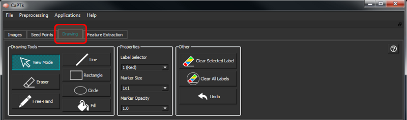
Label Annotation/Drawing Panel
This panel provides the ability to annotate Regions of Interest (ROIs) and save them as masks.
While drawing, you can switch across the image volumes loaded in CaPTk, by pressing the numbers 1-9 on your keyboard.
Toggle between non-zero (taken from the opacity box) and zero opacity of the entire annotated mask by using the keyboard key "m".
Visualize a single label using "Control + <label number>" and add labels to the visualization using "Alt + <label number>". To reset, press "Control/Alt + 0".
There are the following controls underneath the Drawing tab:
| Button/Box | Description |
|---|---|
| View Mode | Switch from drawing mode (which is enabled when either Near or Far ROI drawing is selected) to normal viewing mode |
| Line | Draw a line of selected label color and size |
| Rectangle | Draw a rectangle of selected label color and size |
| Circle | Draw a circle of selected label color and size |
| Sphere | Draw a sphere of selected label color and pre-determined size from the size combo-box |
| Free-Hand | Draw selected label using brush of specified size using mouse left button drag |
| Fill | Fill a closed boundary with selected label - uses ITK's connected component filter |
| Eraser | Erases all labels using brush of specified size |
| Label Selector | Label selector between 1-9 |
| Marker Size | A square marker of specific voxel size |
| Marker Opacity | Sets the opacity of the marker between 0.0 (transparent) and 1.0 (opaque) |
| Clear Selected Label | Remove selected label completely from the mask |
| Clear All Labels | Remove all labels completely from the mask |
| Undo | By providing the same number of old and new values in the format AxBxC, the values of the annotated region can be quickly changed |
| Change Values | By providing the same number of old and new values in the format AxBxC, the values of the annotated region can be quickly changed |
Keyboard Shortcuts
These are the keyboard shortcuts available on CaPTk:
| Key Stroke | Function/Action |
|---|---|
| 1-9 | [IMAGES] Show selected image from table |
| "m" | [DRAWING] Show/Hide all regions; picks up last used opacity |
| Control + 1-9 | [DRAWING] Only show selected label |
| Alt + 1-9 | [DRAWING] Add selected label to visualization |
| Control/Alt + 0 | [DRAWING] Reset label visualization; i.e., show all |
| Shift + Space | [SEED POINT] Set initial tumor center |
| Control + Space | [SEED POINT] Update tumor radius; on macOS, this is "Fn + Command + Space" |
| Space | [SEED POINT] Update tumor center |
Utilities (Command-line only)
To make pipeline construction using CaPTk easier, a bunch of utilities have been provided:
- Resizing
- Resampling
- Image information
- Unique values in image
- Get smallest bounding box in mask (optional isotropic bounding box)
- Test 2 images
- Create mask from threshold
- DICOM to NIfTI conversion
- NIfTI to DICOM & DICOM-Seg conversion
- Re-orient image
- Cast image to another pixel type
- Thresholding:
- Below
- Above
- Above & Below
- Otsu
- Binary
- Convert file formats
- Extract Image Series from Joined stack and vice-versa (4D <-> 3D)
- Transform coordinates from world to image and vice-versa
- Label similarity Metrics between 2 label images: pure mathematical formulations are given as output
- BraTS similarity Metrics between 2 label images: special considerations for metrics are done in this mode because output needs to be BraTS-compliant.
- Collect information from all images in a directory and put it in CSV
For a full list of this functionality and more details, please see the corresponding How-To page.
Pre-processing
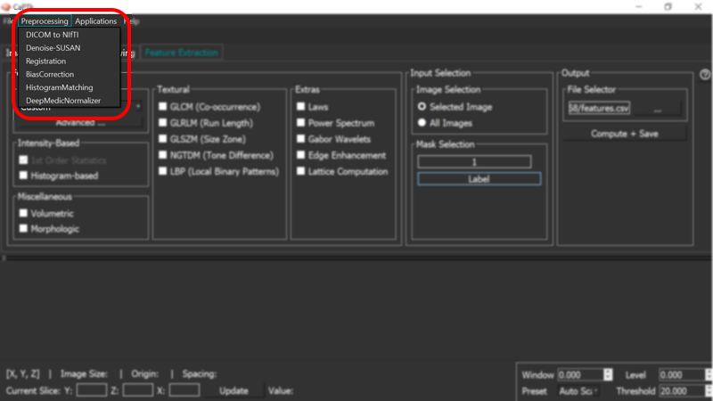
Image pre-processing is essential to quantitative image analysis. CaPTk pre-processing tools available under the "Preprocessing" menu are fully-parameterizable and comprise:
- Denoising. Intensity noise reduction in regions of uniform intensity profile is offered through a low-level image processing method, namely Smallest Univalue Segment Assimilating Nucleus (SUSAN) [1]. This is a custom implementation and does NOT call out to the original implementation distributed by FSL.
- Co-registration. Registration of various images to the same anatomical template, for examining anatomically aligned imaging signals in tandem and at the voxel level, is done using the Greedy Registration algorithm [5].
- Bias correction. Correction for magnetic field inhomogeneity is provided using a non-parametric non-uniform intensity normalization [2].
- Intensity normalization. Conversion of signals across modalities to comparable quantities using histogram matching [4].
- Z-Scoring normalization. Images are normalized using a z-scoring mechanism with option to do the normalization within the region of interest or across the entire image. In addition, there is an option to remove outliers & noise from the image by removing a certain percentage of the top and bottom intensity ranges [6].
- Histogram Matching
- Skull Stripping (Deep Learning based)
- Mammogram Pre-processing
- BraTS Pre-processing Pipeline
NOTE: An extended set of algorithms are available via the command line utility Preprocessing. For full details, run the command:
Preprocessing.exe -u
References:
- S.M.Smith, J.M.Brady, "SUSAN - a new approach to low level image processing", Int. J. Comput. Vis. 23(1):45-78, 1997, DOI:10.102A :1007963824710
- N.J.Tustison, B.B.Avants, P.A.Cook, Y.Zheng, A.Egan, P.A.Yushkevich, J.C.Gee, "N4ITK: Improved N3 Bias Correction", IEEE Trans MeI maging. 29(6):1310-20, 2010, DOI: 10.1109/TMI.2010.2046908
- S.P.Thakur, J.Doshi, S.Pati, S.M.Ha, C.Sako, S.Talbar, U.Kulkarni, C.Davatzikos, G.Erus, S.Bakas, "Brain Extraction on MRI Scans in Presence of Diffuse Glioma: Multi-institutional Performance Evaluation of Deep Learning Methods and Robust Modality-Agnostic Training", NeuroImage 2020, DOI:10.1016/j.neuroimage.2020.117081
- L.G.Nyul, J.K.Udupa, X.Zhang, "New Variants of a Method of MRI Scale Standardization", IEEE Trans Med Imaging. 19(2):143-50, 2000, DOI:10.1109/42.836373
- P.A.Yushkevich, J.Pluta, H.Wang, L.E.Wisse, S.Das, D.Wolk, "Fast Automatic Segmentation of Hippocampal Subfields and Medical Temporal Lobe Subregions in 3 Tesla and 7 Tesla MRI", Alzheimer's & Dementia: The Journal of Alzheimer's Association, 12(7), P126-127, DOI:10.1016/j.jalz.2016.06.205
- T.Rohlfing, N.M.Zahr, E.V.Sullivan, A.Pfefferbaum, "The SRI24 multichannel atlas of normal adult human brain structure", Human Brain Mapping, 31(5):798-819, 2010, DOI:10.1002/hbm.20906
Segmentation
Currently there are two ways to produce segmentation labels for various structures in the images that are loaded:
- using the Geodesic Distance Transform
- using ITK-SNAP
- Skull Stripping (Deep Learning based)
- Tumor Segmentation (Deep Learning based)
More information on how to run those is provided in the corresponding How-To section.
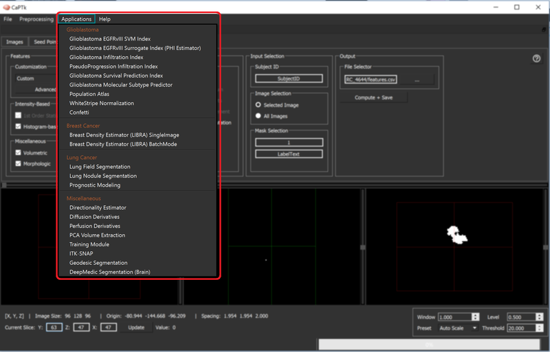
Feature Extraction
The feature extraction tab in CaPTk enables clinicians and other researchers to easily extract feature measurements, commonly used in image analysis, and conduct large-scale analyses in a repeatable manner.
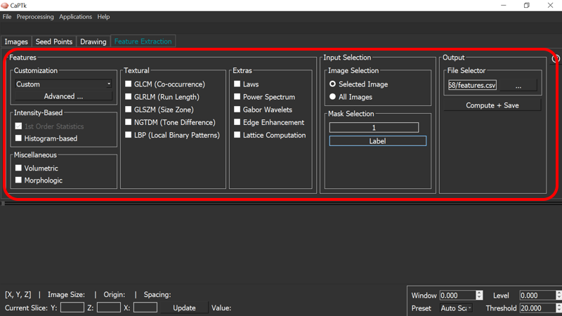
Although the feature panel in CaPTk is continuously expanding, it currently comprises i) intensity-based, ii) textural (GLCM, GLRLM, GLSZM, NGTDM, LBP), and iii) volumetric/morphologic features. You can find the exact list of features incorporated in CaPTk, together with their mathematical definition in the corresponding How-To section.
Specialized applications in CaPTk, such as "EGFRvIII Surrogate Index", "Survival Prediction", "Recurrence Estimator", and "SBRT-Lung" use features of this panel. However, the general idea is to keep the features generic and adaptable for different types of images by just changing the input parameters. Currently we provide some pre-selected parameters for Neuro and Torso images (i.e., Brain, Breast, Lung). Users can alter these pre-selected values through the Custom menu option, or create their own set of parameters via the Advanced menu. The output of the feature extraction tab is a text (.csv) file, with feature names and values. Note that the reported features are extracted per modality, per annotated region and per offset (offset represents the radius around the center pixel; for radius 1, the offset will be +/- 1) value.
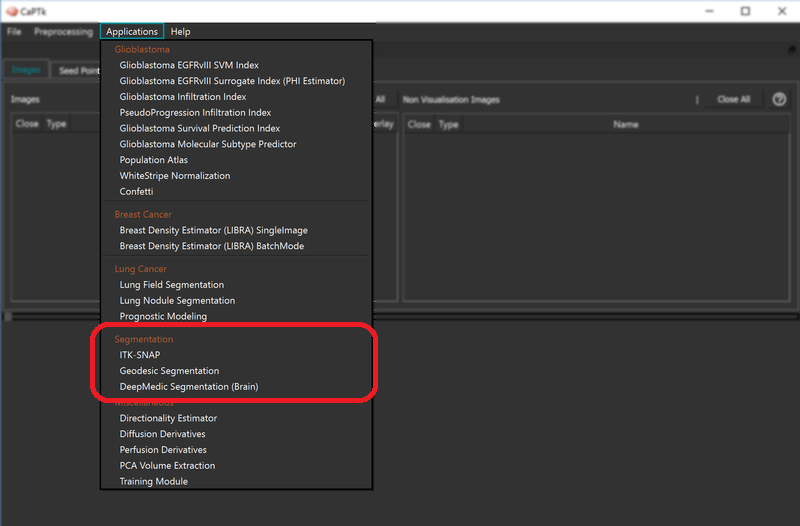
Specialized Applications
Various Specialized Applications are currently incorporated in CaPTk focusing on brain tumors, breast cancer, and lung nodules as shown in the figure below.
For details, please see Specialized Applications (SAs) Usage.
Command Line Usage
Almost every application offered by CaPTk can be used from the command line and utilizing the CaPTk's powerful command line APIs is relatively straight-forward. The following parameters are present in every CLI:
| Laconic | Verbose | Function/Action |
|---|---|---|
| u | usage | Usage message giving all the possible parameters of an application |
| h | help | Help message giving details of parameters (including defaults and ranges) with some examples |
| v | version | The version information of the application |
An example to show the verbose help for an application called ${Application}:
| Platform (x64) | Command |
|---|---|
| Windows | ${CaPTk_InstallDir}/bin/${ApplicationName}.exe -h |
| Linux | ${CaPTk_InstallDir}/bin/${ApplicationName} -h |
| macOS | ~/Applications/CaPTk_${version}.app/Contents/Resources/bin/${ApplicationName} -h |
Detailed explanation of using the command line is available in the How To Guides.